More About How To Vlookup
Youd look in column two if you'd like the scores for Physics. If omitted, it defaults to TRUE approximate match (see additional notes below).Additional Notes (Boring, but important to know)The game could be exact (FALSE or 0 in rangelookup) or approximate (TRUE or 1).In approximate search, make sure the listing is sorted in ascending sequence (top to bottom), or the outcome could be wrong.
If the lookupvalue is bigger than the value, it returns a # N/A error. If lookupvalue is text, wildcard characters can be used (refer to the case below).Now, trusting that you have a basic comprehension of what the VLOOKUP function could do, lets peel this onion and see some useful examples of the VLOOKUP function.


The Definitive Guide to How To Use Vlookup In Excel
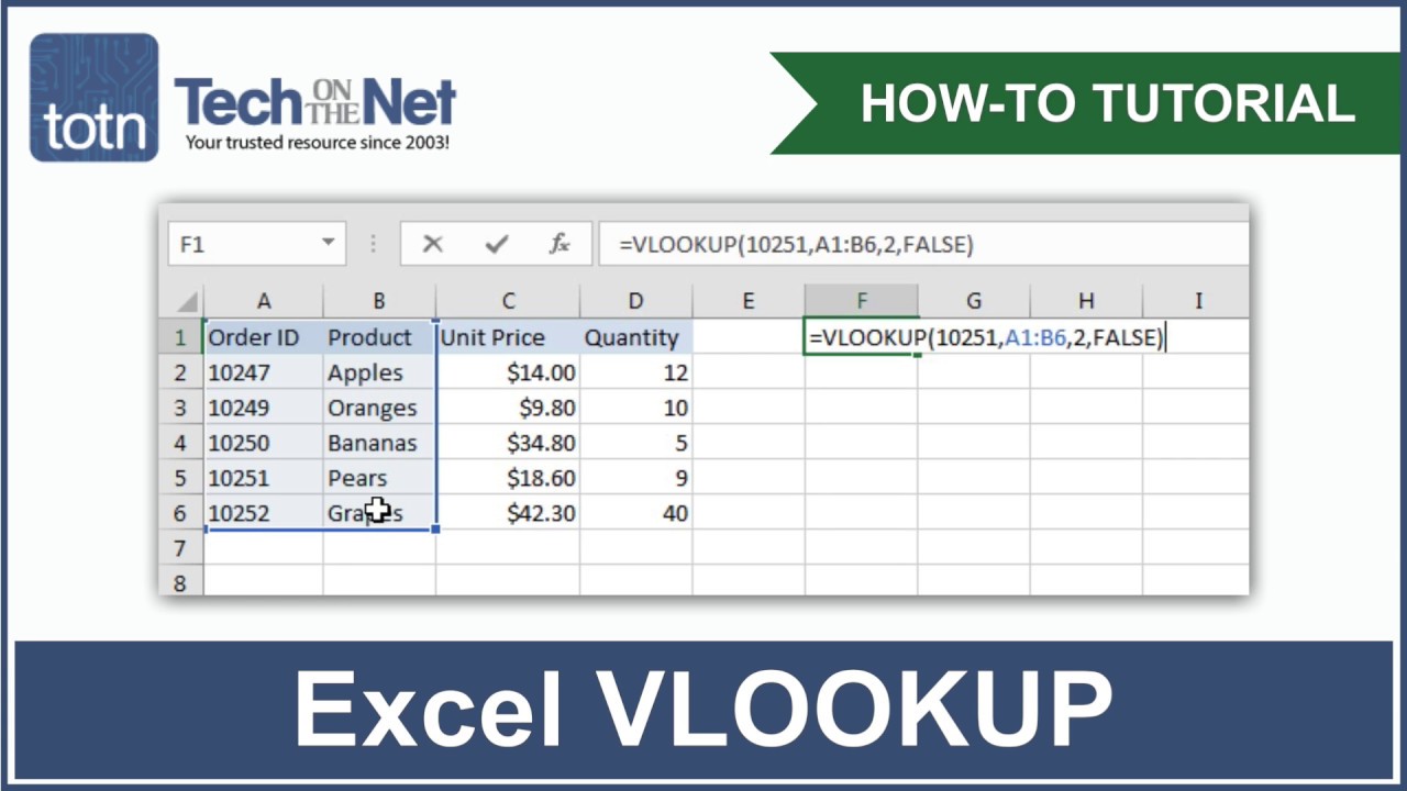
0 tells the VLOOKUP function to look for exact matches. Here is the way the above example is worked in by the VLOOKUP formula. It looks for its worth Brad from the left-most column. It goes at the top to bottom and also discovers the value in mobile A 6. The moment that the value is found by it, it brings the value within it and extends to the right from the next column.
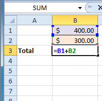
You may also use a cell reference that comprises the lookup value. The advantage of utilizing a cell reference is that it makes the formulation lively.
Since we've employed two Thus, the formulation would always return the score for Math. However, what if you wish to make both the VLOOKUP the column index number energetic along with value.
This is a good example of a VLOOKUP formula. This is a good illustration of a two-way VLOOKUP function. useful source You have to create the column dynamic, to make this two-way lookup formula. So when a user changes the subject, the formula automatically selects the correct column (two in the case of Math, 3 in the case of Physics, etc. .) .To do so, you want to use the MATCH function as the pillar argument.
More About Excel Vlookup Function
MATCH function requires the domain as the search value (in H 3) and returns its place in Part 2:E 2. Therefore, if you employ Math, it might yield two as Math can be located in B 2 (that is the next cell in the specified array range).Example 3 Using Drop Down Lists as Lookup Values In the above example, we have to manually enter the data.
A good idea in such cases is to create a drop-down list of the lookup values (in this scenario, it might be student names and subjects) and then simply choose from the listing. Depending on the selection, the formula would automatically update the outcome. A thing as shown below:This creates a fantastic dashboard component as you can have a massive data set with countless pupils at the rear end, however the end user (lets say a teacher) can quickly receive the marks of a student in a topic by simply creating the selections from the drop down.
Here are the steps the cell where you would like the drop-down listing. In this example, in G , we want the student titles. Go to Data Data Tools Data Validation. Inside the settings tab , in the Data Validation Dialogue box, select List from the drop-down.
Similarly, one can be created by you in H 3. Instance 4 Three-way Lookup What is a research In Example 2, weve employed one lookup table in various subjects with scores for all pupils. This is a good instance of a two-way lookup as we use two variables to bring the score (students name and the topics title ). Now, suppose in a visit this page calendar year, a pupil has three distinct levels of examinations, Unit Evaluation, Midterm, and Final Evaluation (thats exactly what I've had when I was a pupil ). A three-way lookup are able to get a students marks for a predetermined subject from the my review here level of examination.